WRITER Dr Jeremy CK Tan

Standard automated perimetry (SAP) remains the primary method for assessing functional loss in glaucoma.1 The threshold visual field (VF) test report typically contains a large number of summary and detailed metrics that describe the sensitivity and reliability properties of the test, such as the mean deviation (MD) and the threshold sensitivity of grid locations.

In this article, Dr Jeremy Tan provides some guidance on interpreting these metrics.

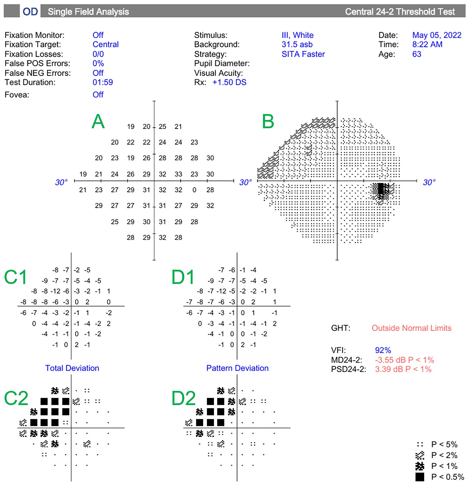
Figure 1. An example of a Humphrey Field Analyser visual field report of a patient’s right eye, using the SITA-Faster strategy. The various plots are labelled in green as follows: A) numerical sensitivity plot, B) grayscale plot, C) total deviation plot (shown with numerical values (C1) and probability values (C2)), pattern deviation plot (shown with numerical (D1) and probability values (D2)). The global reliability and sensitivity indices are also displayed on the report.

The outputs provided on the typical VF test reports are assessed by the clinician for two common scenarios:

1. Diagnosis; to determine if a glaucomatous or non-glaucomatous VF defect is present,

2. Progression; if the VF has progressed compared to previous tests.

Interpretation of the VF report can be challenging not only because of the number of data points being presented but because the variability of testing can add uncertainty on what is pathology versus artefact. A systematic approach to working through the numerous data points is therefore often helpful in ensuring pertinent information is not missed. This article outlines the clinical interpretation of the visual field using the Humphrey Field Analyser single field report as an example. The various plots displayed and the main sensitivity and reliability indices will be discussed.

The numerical plot (Figure 1, plot A) is a grid of numbers that represent the ‘raw’ sensitivities measured at each test location. In the Humphrey 24-2 program, a total of 54 stimulus locations are presented. This consists of 52 test points, which are used in the deviation plots and global indices, and two blind spot locations. The associated grayscale plot (Figure 1, plot B) is generated from the numerical values. Darker shading indicates areas of lower sensitivity and therefore a greater visual field defect, while lighter shading represents more preserved sensitivity.

Total Deviation

The total deviation plot shows the difference in sensitivity at each test location compared with age- and location-matched normal values, expressed in decibels (Figure 1, plot C1). Probability symbols beneath each point indicate how likely such a deviation would be in a normal population, with darker symbols representing more statistically significant abnormalities (Figure 1, plot C2).

Global sensitivity indices refer to a set of summary (global) statistics that capture information relating to the amount of VF loss, and whether the VF loss is generalised or focal.

The MD is perhaps the most commonly used global sensitivity index on the VF report, and accounts for both age and eccentricity of test locations. It is the average difference between measured threshold sensitivities of all locations on the test grid, and an age-corrected normal reference field. More weight is given to certain values when computing the final average, as certain VF locations are known to provide more reliable estimates of sensitivity.2

The MD reflects the overall degree of depression in the VF and is expressed in decibels. More negative values indicate greater field loss, and the MD value is often used in clinical practice to classify disease severity at baseline. While multiple classification systems exist,3 a commonly used rule is to define mild severity as an MD value between 0 and -6 dB, moderate as between -12 to -6 dB, and severe as MD below -12 dB.

Figure 2. Examples of glaucomatous visual fields of the right eye with increasing severity. Each row shows the total deviation map (left) and the corresponding pattern deviation probability plot (right). A) Inferior nasal step defect (MD –4.50 dB). B) inferior arcuate defect (MD –8.00 dB). C) Advanced generalised loss with diffuse depression across the field (MD –21.60 dB). In the pattern deviation probability plots, the shaded red boxes represent test locations where sensitivity loss is statistically significant compared with an age-matched normal population, with darker shading indicating greater depth and significance of defect.

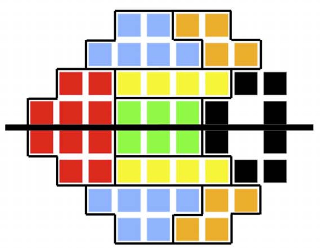
Figure 3: Five pairs of colour-coded visual field sectors used in the glaucoma hemifield test, compared across the horizontal meridian to assess asymmetry. Used with permission from Phu et al., 2018.5Figure 3: Five pairs of colour-coded visual field sectors used in the glaucoma hemifield test, compared across the horizontal meridian to assess asymmetry. Used with permission from Phu et al., 2018.5

Pattern Deviation

The pattern deviation plot adjusts the total deviation values by removing any generalised depression or elevation in sensitivity (e.g., from cataract or small pupil), thereby highlighting localised defects (Figure 1, plot D1). Probability symbols indicate the statistical significance of these residual deviations, making it easier to distinguish true focal loss from diffuse changes (Figure 1, plot D2). The probability symbols on the total and pattern deviation plots are accompanied by a legend (5%, 2%, 1%, and 0.5%), which represent statistical significance thresholds compared with an age-matched normal population. For example, a black square at <0.5% indicates that fewer than one in 200 normal eyes would be expected to show such a deviation, making it highly suspicious for true visual field loss.

Unlike the MD, which reflects overall loss, pattern standard deviation (PSD) measures localised visual field changes. The PSD is derived after removing any generalised depression or elevation, leaving only the localised deviations in the field.

It is calculated as the root mean square of these values, providing a measure of average irregularity – where higher PSD indicates greater focal loss. A higher PSD therefore indicates greater localised variation in sensitivity, whereas a low PSD suggests a more uniform field – whether normal or diffusely depressed in advanced disease.

Figure 2 illustrates examples of glaucomatous visual fields across a spectrum of severity. In each case, the total deviation map is shown alongside the corresponding pattern deviation probability plot. The examples demonstrate a mild localised defect (MD –4.50 dB), a moderate arcuate defect (MD –8.00 dB), and advanced diffuse loss (MD –21.60 dB). In the probability plots, shaded red boxes denote test locations with statistically significant sensitivity loss relative to an age-matched normative database, with darker shading reflecting greater depth and significance of the defect.

Visual Field Index

The visual field index (VFI), much like the MD, is a summary measure of generalised field loss. However, it places greater emphasis on central test locations and is designed to reflect functional vision more accurately in the context of glaucoma. The VFI is expressed as a percentage, with 100% representing normal age-corrected function and 0% indicating total field loss. It is derived by identifying points considered abnormal, based on pattern and total deviation probability maps. Only points outside normal limits are included in the calculation, and these are weighted more heavily if they are located centrally.2 The VFI calculation reduces the influence of diffuse media opacities such as cataract.

Glaucoma Hemifield Test

The Humphrey Field Analyser (HFA) also reports the glaucoma hemifield test (GHT), an automated index developed to detect glaucomatous visual field loss. The GHT compares five pairs of anatomically matched sectors in the superior and inferior hemifields, mirrored across the horizontal meridian, based on the normal course of the retinal nerve fibre layer. For each pair, it assesses the difference in abnormality probability scores.4 These differences are compared to empirically determined limits from healthy eyes: a result is outside normal limits if any difference exceeds the 99th percentile of normal values (i.e., larger than all but the most extreme 1% in the normal population), within normal limits if all differences are within the 97th percentile, and borderline if the differences fall in between. The GHT can also detect generalised sensitivity loss or abnormally high sensitivities and prints a brief text summary on the VF report (Figure 3).

Computerised perimetry was initially implemented with three parameters to help users evaluate the reliability and usefulness of test results: fixation losses (FL), false negative rate (FN), and false positive rate (FP).6

Fixation Losses

Fixation losses (FL) were originally determined using the Heijl–Krakau method, where stimuli were presented within the expected location of the physiologic blind spot. Their accuracy, however, is affected by incorrect mapping of the blind spot or if the head is tilted/moved during testing. With the release of gaze tracking, the FL index has become less important in assessing fixation during testing.

False Negative Rate

False negative (FN) responses are obtained by re-presenting suprathreshold stimuli above a threshold established earlier in the test, and act as a surrogate for inattention. FN responses may, however, be influenced more by the level of visual field damage than on patient vigilance,7,8 where extensive visual field loss increases the uncertainty of whether a stimulus was actually seen. A high FN rate should therefore not automatically mean the test is unreliable.

False Positive Rate

False positive (FP) responses are intended to identify ‘trigger happy’ behaviour and were originally measured using catch trials in a response window in which no stimulus was presented. Modern strategies on the Humphrey, however, estimate FP based on the detection of patient responses during intervals where it is impossible or unlikely for a stimulus to have been seen.6 The 15% threshold is often used as a criterion for reliability, however this threshold may be closer to 33% in the new SITA-Faster strategy.9 Clinicians should therefore not automatically disregard fields with FP >15%, especially if the test appears reliable on clinical inspection.

Gaze tracking (GT) measures degrees of gaze deviation during stimulus presentation and reports GT failures in real time.10 GT outputs are displayed as upward bars that are representative of gaze deviations, with increasing bar sizes indicative of larger gaze deviations, while downward bars indicate failure to capture a signal.10 The association between standard reliability metrics and gaze tracking metrics is however unclear;10,11 therefore GT outputs cannot be relied upon to assess test reliability.

VF interpretation is essential in glaucoma care yet can be difficult due to the number and complexity of indices presented. The reliability of a test report is often assessed first, and while the importance of FL and FN in assessing test reliability has declined over time, FP responses remain widely used in modern perimetric strategies. The global sensitivity indices, as described above, are then used to summarise the overall severity of VF loss (MD and VFI), while PSD reflects whether the loss is localised, and GHT assesses whether the pattern is consistent with glaucomatous damage. While each parameter has limitations, a systematic approach to interpreting the VF threshold report may assist clinicians to ascertain key features.

Dr Jeremy CK Tan is an ophthalmologist practising in Sydney. He is a staff specialist ophthalmologist at the Prince of Wales Hospital Randwick and the director of Horizon Eye Specialists, Sydney. He has research interests in visual fields testing, glaucoma
surgery and ophthalmic imagine.

References available at mivision.com.au.